Finding the critical value is essential in hypothesis testing to determine whether to reject the null hypothesis. At how.edu.vn, we understand the importance of accurate statistical analysis, and we’re here to provide you with expert guidance. Whether you’re dealing with z-values, t-values, chi-square values, or f-values, understanding how to find and use critical values is crucial for making informed decisions. This article will explore critical values, their formulas, and methods for calculating them, enhanced by the expertise of our team of over 100 distinguished Ph.D. experts.
1. Understanding Critical Values
A critical value is a threshold that helps decide whether to reject the null hypothesis. In hypothesis testing, you compare your test statistic to this critical value. If the absolute value of your test statistic exceeds the critical value, the results are statistically significant, indicating that the null hypothesis can be rejected. This concept is foundational in statistical analysis, ensuring decisions are based on robust evidence.
1.1. Types of Critical Value Tests
Depending on the nature of your hypothesis, different types of tests require different approaches:
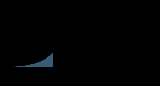
- Left-Tailed Test: This test checks if the statistic is significantly less than a certain value. The critical value is denoted as Q(α).
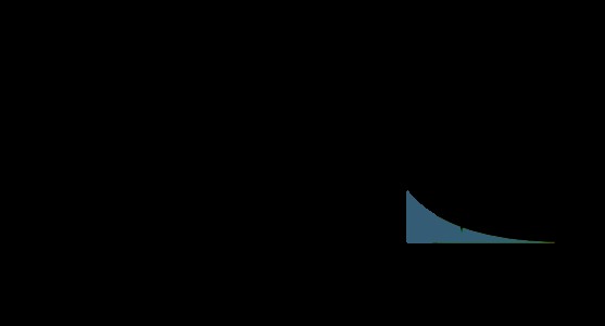
- Right-Tailed Test: This test determines if the statistic is significantly greater than a certain value. The critical value is Q(1 – α).
- Two-Tailed Test: This test checks if the statistic is significantly different from a certain value (either greater or less). The critical values are Q(α/2) ∪ Q(1 – α/2).
2. T Critical Value
The t critical value is a point that defines the cutoff in a Student’s t-distribution. It is used to compare against a calculated t-score in hypothesis testing. Determining the t critical value assists in deciding whether to support or reject a null hypothesis.
2.1. Key Features of T Critical Value
- Used when the sample size is small or the population standard deviation is unknown.
- The t-distribution is symmetrical and bell-shaped, similar to the standard normal distribution but with heavier tails.
- The shape of the t-distribution depends on the degrees of freedom (df), which is typically n-1, where n is the sample size.
3. Z Critical Value
The z critical value is a point that defines an area under the standard normal distribution. This value helps determine the probability of a particular variable occurring. The z and t critical values are quite similar, especially with larger sample sizes.
3.1. Importance of Z Critical Value
- Used when the sample size is large and the population standard deviation is known.
- The z-value represents how many standard deviations away from the mean a particular data point is.
- It is widely used in various statistical tests, including hypothesis testing and confidence intervals.
4. F Critical Value
The F critical value is a threshold at which the probability α of a Type-I error occurs (mistakenly rejecting a true null hypothesis). The F statistic is derived from the F-distribution table and is commonly used in tests such as ANOVA and regression analysis.
4.1. Applications of F Critical Value
- ANOVA (Analysis of Variance): Used to compare means across multiple groups.
- Overall Significance in Regression Analysis: Determines if the model as a whole is statistically significant.
- Comparing Nested Regression Models: Assesses whether adding additional predictors significantly improves the model.
- Equality of Variances in Two Normally Distributed Populations: Tests whether the variances of two populations are equal.
Our F critical value calculator simplifies this process, providing accurate values with a single click.
5. Chi-Square Value
Chi-square values serve as thresholds for statistical significance in certain hypothesis tests and confidence intervals. These values are evaluated using the Chi-square distribution table.
5.1. Uses of Chi-Square Value
- Goodness-of-Fit Tests: Determines if a sample data matches a population.
- Homogeneity Tests: Checks if different samples come from the same population.
- Tests for Independence in Contingency Tables: Evaluates if two categorical variables are independent.
Unlike t and F critical values, the chi-square critical value requires specifying the degrees of freedom to obtain the result.
6. Critical Value Formulas
Understanding the formulas behind critical values can deepen your comprehension of statistical testing. Here are the formulas for z and t critical values:
| Type of Critical Value | T Critical Value Formula | Z Critical Value Formula |
|---|---|---|
| Left-Tailed | Qt,d(α) | u(α) |
| Right-Tailed | Qt,d(1 – α) | u(1 – α) |
| Two-Tailed | ±Qt,d(1 – α/2) | ±u(1 – α/2) |

Where:
- Qt is the quantile function of the t-student distribution.
- u is the quantile function of the normal distribution.
- d refers to the degrees of freedom.
- α is the significance level.
A t critical value calculator uses these formulas to deliver the exact critical values needed to accept or reject a hypothesis.
7. Finding Critical Values Manually
Although calculators simplify the process, knowing How To Find Critical Values manually is beneficial. This section provides examples for both t and z critical values.
7.1. How to Find T Critical Value
Example:
Find the t critical value if the sample size is 5 and the significance level is 0.05.
Solution:
Step 1:
Subtract 1 from the sample size to get the degrees of freedom.
Degree of Freedom = N – 1 = 5 – 1
Degree of freedom = 4
α = 0.05
Step 2:
Choose the appropriate t-distribution table (one-tailed or two-tailed) based on your test.
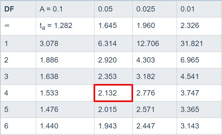
Step 3:
Locate the degrees of freedom in the leftmost column and the significance level α in the top row. The value at their intersection is the t critical value.
In this case, the t critical value is 2.132.
7.2. How to Find Z Critical Value
Example:
Find the z critical value if the significance level is 0.02.
Solution:
Step 1:
Divide the significance level α by 2.
α/2 = 0.02 / 2
α/2 = 0.01
Step 2:
Subtract α/2 from 1.
1 – α/2 = 1 – 0.01
1 – α/2 = 0.99
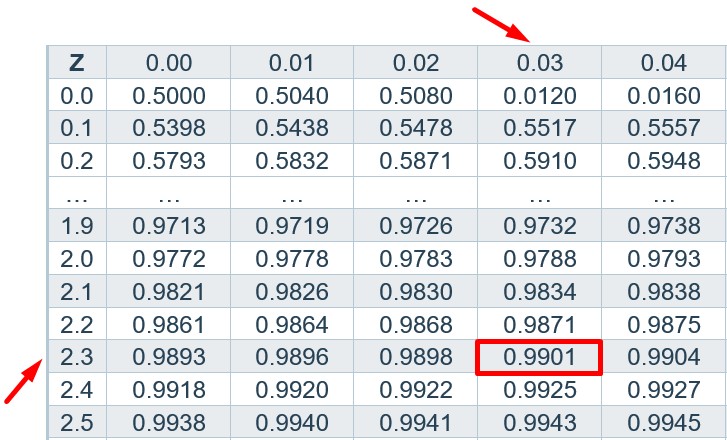
Step 3:
Search for the value 0.99 in the z table. Add the values of the intersecting row (top) and column (most left) to get the z critical value.
- 3 + 0.03 = 2.33
Z critical value = ±2.33 for the two-tailed test.
8. T-Distribution Table (One Tail)
The t-distribution table for one-tail probability is provided below.
[Download Table]
| DF | A = 0.1 | 0.05 | 0.025 | 0.01 | 0.005 | 0.001 | 0.0005 |
|---|---|---|---|---|---|---|---|
| ∞ | 1.282 | 1.645 | 1.960 | 2.326 | 2.576 | 3.091 | 3.291 |
| 1 | 3.078 | 6.314 | 12.706 | 31.821 | 63.656 | 318.289 | 636.578 |
| 2 | 1.886 | 2.920 | 4.303 | 6.965 | 9.925 | 22.328 | 31.600 |
| 3 | 1.638 | 2.353 | 3.182 | 4.541 | 5.841 | 10.214 | 12.924 |
| 4 | 1.533 | 2.132 | 2.776 | 3.747 | 4.604 | 7.173 | 8.610 |
| 5 | 1.476 | 2.015 | 2.571 | 3.365 | 4.032 | 5.894 | 6.869 |
| 6 | 1.440 | 1.943 | 2.447 | 3.143 | 3.707 | 5.208 | 5.959 |
| 7 | 1.415 | 1.895 | 2.365 | 2.998 | 3.499 | 4.785 | 5.408 |
| 8 | 1.397 | 1.860 | 2.306 | 2.896 | 3.355 | 4.501 | 5.041 |
| 9 | 1.383 | 1.833 | 2.262 | 2.821 | 3.250 | 4.297 | 4.781 |
| 10 | 1.372 | 1.812 | 2.228 | 2.764 | 3.169 | 4.144 | 4.587 |
| 11 | 1.363 | 1.796 | 2.201 | 2.718 | 3.106 | 4.025 | 4.437 |
| 12 | 1.356 | 1.782 | 2.179 | 2.681 | 3.055 | 3.930 | 4.318 |
| 13 | 1.350 | 1.771 | 2.160 | 2.650 | 3.012 | 3.852 | 4.221 |
| 14 | 1.345 | 1.761 | 2.145 | 2.624 | 2.977 | 3.787 | 4.140 |
| 15 | 1.341 | 1.753 | 2.131 | 2.602 | 2.947 | 3.733 | 4.073 |
| 16 | 1.337 | 1.746 | 2.120 | 2.583 | 2.921 | 3.686 | 4.015 |
| 17 | 1.333 | 1.740 | 2.110 | 2.567 | 2.898 | 3.646 | 3.965 |
| 18 | 1.330 | 1.734 | 2.101 | 2.552 | 2.878 | 3.610 | 3.922 |
| 19 | 1.328 | 1.729 | 2.093 | 2.539 | 2.861 | 3.579 | 3.883 |
| 20 | 1.325 | 1.725 | 2.086 | 2.528 | 2.845 | 3.552 | 3.850 |
| 21 | 1.323 | 1.721 | 2.080 | 2.518 | 2.831 | 3.527 | 3.819 |
| 22 | 1.321 | 1.717 | 2.074 | 2.508 | 2.819 | 3.505 | 3.792 |
| 23 | 1.319 | 1.714 | 2.069 | 2.500 | 2.807 | 3.485 | 3.768 |
| 24 | 1.318 | 1.711 | 2.064 | 2.492 | 2.797 | 3.467 | 3.745 |
| 25 | 1.316 | 1.708 | 2.060 | 2.485 | 2.787 | 3.450 | 3.725 |
| 26 | 1.315 | 1.706 | 2.056 | 2.479 | 2.779 | 3.435 | 3.707 |
| 27 | 1.314 | 1.703 | 2.052 | 2.473 | 2.771 | 3.421 | 3.689 |
| 28 | 1.313 | 1.701 | 2.048 | 2.467 | 2.763 | 3.408 | 3.674 |
| 29 | 1.311 | 1.699 | 2.045 | 2.462 | 2.756 | 3.396 | 3.660 |
| 30 | 1.310 | 1.697 | 2.042 | 2.457 | 2.750 | 3.385 | 3.646 |
| 60 | 1.296 | 1.671 | 2.000 | 2.390 | 2.660 | 3.232 | 3.460 |
| 120 | 1.289 | 1.658 | 1.980 | 2.358 | 2.617 | 3.160 | 3.373 |
| 1000 | 1.282 | 1.646 | 1.962 | 2.330 | 2.581 | 3.098 | 3.300 |
9. T-Distribution Table (Two Tail)
The t-distribution table for two-tail probability is provided below.
[Download Table]
| DF | A = 0.2 | 0.10 | 0.05 | 0.02 | 0.01 | 0.002 | 0.001 |
|---|---|---|---|---|---|---|---|
| ∞ | 1.282 | 1.645 | 1.960 | 2.326 | 2.576 | 3.091 | 3.291 |
| 1 | 3.078 | 6.314 | 12.706 | 31.821 | 63.656 | 318.289 | 636.578 |
| 2 | 1.886 | 2.920 | 4.303 | 6.965 | 9.925 | 22.328 | 31.600 |
| 3 | 1.638 | 2.353 | 3.182 | 4.541 | 5.841 | 10.214 | 12.924 |
| 4 | 1.533 | 2.132 | 2.776 | 3.747 | 4.604 | 7.173 | 8.610 |
| 5 | 1.476 | 2.015 | 2.571 | 3.365 | 4.032 | 5.894 | 6.869 |
| 6 | 1.440 | 1.943 | 2.447 | 3.143 | 3.707 | 5.208 | 5.959 |
| 7 | 1.415 | 1.895 | 2.365 | 2.998 | 3.499 | 4.785 | 5.408 |
| 8 | 1.397 | 1.860 | 2.306 | 2.896 | 3.355 | 4.501 | 5.041 |
| 9 | 1.383 | 1.833 | 2.262 | 2.821 | 3.250 | 4.297 | 4.781 |
| 10 | 1.372 | 1.812 | 2.228 | 2.764 | 3.169 | 4.144 | 4.587 |
| 11 | 1.363 | 1.796 | 2.201 | 2.718 | 3.106 | 4.025 | 4.437 |
| 12 | 1.356 | 1.782 | 2.179 | 2.681 | 3.055 | 3.930 | 4.318 |
| 13 | 1.350 | 1.771 | 2.160 | 2.650 | 3.012 | 3.852 | 4.221 |
| 14 | 1.345 | 1.761 | 2.145 | 2.624 | 2.977 | 3.787 | 4.140 |
| 15 | 1.341 | 1.753 | 2.131 | 2.602 | 2.947 | 3.733 | 4.073 |
| 16 | 1.337 | 1.746 | 2.120 | 2.583 | 2.921 | 3.686 | 4.015 |
| 17 | 1.333 | 1.740 | 2.110 | 2.567 | 2.898 | 3.646 | 3.965 |
| 18 | 1.330 | 1.734 | 2.101 | 2.552 | 2.878 | 3.610 | 3.922 |
| 19 | 1.328 | 1.729 | 2.093 | 2.539 | 2.861 | 3.579 | 3.883 |
| 20 | 1.325 | 1.725 | 2.086 | 2.528 | 2.845 | 3.552 | 3.850 |
| 21 | 1.323 | 1.721 | 2.080 | 2.518 | 2.831 | 3.527 | 3.819 |
| 22 | 1.321 | 1.717 | 2.074 | 2.508 | 2.819 | 3.505 | 3.792 |
| 23 | 1.319 | 1.714 | 2.069 | 2.500 | 2.807 | 3.485 | 3.768 |
| 24 | 1.318 | 1.711 | 2.064 | 2.492 | 2.797 | 3.467 | 3.745 |
| 25 | 1.316 | 1.708 | 2.060 | 2.485 | 2.787 | 3.450 | 3.725 |
| 26 | 1.315 | 1.706 | 2.056 | 2.479 | 2.779 | 3.435 | 3.707 |
| 27 | 1.314 | 1.703 | 2.052 | 2.473 | 2.771 | 3.421 | 3.689 |
| 28 | 1.313 | 1.701 | 2.048 | 2.467 | 2.763 | 3.408 | 3.674 |
| 29 | 1.311 | 1.699 | 2.045 | 2.462 | 2.756 | 3.396 | 3.660 |
| 30 | 1.310 | 1.697 | 2.042 | 2.457 | 2.750 | 3.385 | 3.646 |
| 60 | 1.296 | 1.671 | 2.000 | 2.390 | 2.660 | 3.232 | 3.460 |
| 120 | 1.289 | 1.658 | 1.980 | 2.358 | 2.617 | 3.160 | 3.373 |
| ∞ | 1.282 | 1.645 | 1.960 | 2.326 | 2.576 | 3.091 | 3.291 |
10. Z Table (Right-Tailed)
The normal distribution table for the right-tailed test is provided below.
[Download Table]
| Z | 0.00 | 0.01 | 0.02 | 0.03 | 0.04 | 0.05 | 0.06 | 0.07 | 0.08 | 0.09 |
|---|---|---|---|---|---|---|---|---|---|---|
| 0.0 | 0.0000 | 0.0040 | 0.0080 | 0.0120 | 0.0160 | 0.0199 | 0.0239 | 0.0279 | 0.0319 | 0.0359 |
| 0.1 | 0.0398 | 0.0438 | 0.0478 | 0.0517 | 0.0557 | 0.0596 | 0.0636 | 0.0675 | 0.0714 | 0.0753 |
| 0.2 | 0.0793 | 0.0832 | 0.0871 | 0.0910 | 0.0948 | 0.0987 | 0.1026 | 0.1064 | 0.1103 | 0.1141 |
| 0.3 | 0.1179 | 0.1217 | 0.1255 | 0.1293 | 0.1331 | 0.1368 | 0.1406 | 0.1443 | 0.1480 | 0.1517 |
| 0.4 | 0.1554 | 0.1591 | 0.1628 | 0.1664 | 0.1700 | 0.1736 | 0.1772 | 0.1808 | 0.1844 | 0.1879 |
| 0.5 | 0.1915 | 0.1950 | 0.1985 | 0.2019 | 0.2054 | 0.2088 | 0.2123 | 0.2157 | 0.2190 | 0.2224 |
| 0.6 | 0.2257 | 0.2291 | 0.2324 | 0.2357 | 0.2389 | 0.2422 | 0.2454 | 0.2486 | 0.2517 | 0.2549 |
| 0.7 | 0.2580 | 0.2611 | 0.2642 | 0.2673 | 0.2704 | 0.2734 | 0.2764 | 0.2794 | 0.2823 | 0.2852 |
| 0.8 | 0.2881 | 0.2910 | 0.2939 | 0.2967 | 0.2995 | 0.3023 | 0.3051 | 0.3078 | 0.3106 | 0.3133 |
| 0.9 | 0.3159 | 0.3186 | 0.3212 | 0.3238 | 0.3264 | 0.3289 | 0.3315 | 0.3340 | 0.3365 | 0.3389 |
| 1.0 | 0.3413 | 0.3438 | 0.3461 | 0.3485 | 0.3508 | 0.3531 | 0.3554 | 0.3577 | 0.3599 | 0.3621 |
| 1.1 | 0.3643 | 0.3665 | 0.3686 | 0.3708 | 0.3729 | 0.3749 | 0.3770 | 0.3790 | 0.3810 | 0.3830 |
| 1.2 | 0.3849 | 0.3869 | 0.3888 | 0.3907 | 0.3925 | 0.3944 | 0.3962 | 0.3980 | 0.3997 | 0.4015 |
| 1.3 | 0.4032 | 0.4049 | 0.4066 | 0.4082 | 0.4099 | 0.4115 | 0.4131 | 0.4147 | 0.4162 | 0.4177 |
| 1.4 | 0.4192 | 0.4207 | 0.4222 | 0.4236 | 0.4251 | 0.4265 | 0.4279 | 0.4292 | 0.4306 | 0.4319 |
| 1.5 | 0.4332 | 0.4345 | 0.4357 | 0.4370 | 0.4382 | 0.4394 | 0.4406 | 0.4418 | 0.4429 | 0.4441 |
| 1.6 | 0.4452 | 0.4463 | 0.4474 | 0.4484 | 0.4495 | 0.4505 | 0.4515 | 0.4525 | 0.4535 | 0.4545 |
| 1.7 | 0.4554 | 0.4564 | 0.4573 | 0.4582 | 0.4591 | 0.4599 | 0.4608 | 0.4616 | 0.4625 | 0.4633 |
| 1.8 | 0.4641 | 0.4649 | 0.4656 | 0.4664 | 0.4671 | 0.4678 | 0.4686 | 0.4693 | 0.4699 | 0.4706 |
| 1.9 | 0.4713 | 0.4719 | 0.4726 | 0.4732 | 0.4738 | 0.4744 | 0.4750 | 0.4756 | 0.4761 | 0.4767 |
| 2.0 | 0.4772 | 0.4778 | 0.4783 | 0.4788 | 0.4793 | 0.4798 | 0.4803 | 0.4808 | 0.4812 | 0.4817 |
| 2.1 | 0.4821 | 0.4826 | 0.4830 | 0.4834 | 0.4838 | 0.4842 | 0.4846 | 0.4850 | 0.4854 | 0.4857 |
| 2.2 | 0.4861 | 0.4864 | 0.4868 | 0.4871 | 0.4875 | 0.4878 | 0.4881 | 0.4884 | 0.4887 | 0.4890 |
| 2.3 | 0.4893 | 0.4896 | 0.4898 | 0.4901 | 0.4904 | 0.4906 | 0.4909 | 0.4911 | 0.4913 | 0.4916 |
| 2.4 | 0.4918 | 0.4920 | 0.4922 | 0.4925 | 0.49 |