How to Use VLOOKUP in Excel: A Comprehensive Guide

Microsoft Excel’s VLOOKUP function is a powerful tool for data analysis, allowing you to search for specific information within a table or dataset. Whether you need to find a price based on a product ID, retrieve a customer name using their account number, or match data across different spreadsheets, VLOOKUP can significantly streamline your workflow. This guide will provide you with a step-by-step understanding of how to effectively use VLOOKUP in Excel, making data lookup tasks efficient and accurate.

Understanding VLOOKUP and When to Use It

VLOOKUP, which stands for “Vertical Lookup,” is designed to search for a value in the first column of a table and return a corresponding value from a column to the right within the same row. It’s invaluable when you have large datasets and need to quickly find related information without manually sifting through rows and columns.

Here are common scenarios where VLOOKUP is particularly useful:

Price Lists: Looking up the price of an item based on its product code.
Employee Directories: Finding an employee’s department or contact information using their employee ID.
Inventory Management: Checking stock levels or locations based on product names or SKUs.
Data Matching: Combining data from different spreadsheets by matching common identifiers.
Gradebooks: Assigning grades based on score ranges.

Key Concept: VLOOKUP works vertically, meaning it searches downwards in the first column of your specified table to find the lookup value. The data you want to retrieve must be located in a column to the right of this first column.

VLOOKUP Syntax Explained

The VLOOKUP function uses a specific syntax with four arguments, as follows:

=VLOOKUP(lookup_value, table_array, col_index_num, [range_lookup])

Let’s break down each argument:

lookup_value (required): This is the value you are searching for. It can be a number, text string, or a cell reference. This value must be present in the first column of your table_array.
table_array (required): This is the range of cells that contains the table where you want to search and retrieve data. It should include the column containing your lookup_value (as the first column) and the column containing the value you want to return. You can use cell ranges (e.g., A2:D10), named ranges, or even table names for this argument.
col_index_num (required): This is the column index number within your table_array from which you want to retrieve the matching value. The column index starts from 1, referring to the first column of your table_array. For example, if your table_array is B2:E7, column B is index 1, column C is index 2, column D is index 3, and column E is index 4.
[range_lookup] (optional): This argument specifies whether you want to find an exact match or an approximate match. It accepts two logical values:
- TRUE or 1 (Approximate Match): VLOOKUP will look for the closest match less than or equal to the lookup_value. Crucially, if you use TRUE or omit this argument, the first column of your table_array must be sorted in ascending order. If not sorted, you might get incorrect or unexpected results. This is the default behavior if you don’t specify range_lookup.
- FALSE or 0 (Exact Match): VLOOKUP will only find an exact match for the lookup_value. If an exact match is not found, VLOOKUP will return the #N/A error. This is generally the more commonly used and safer option, especially when dealing with text or unique identifiers.

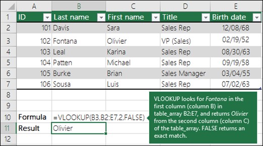
Alt text: VLOOKUP formula example in Excel showing lookup value “Fontana”, table array B2:E7, column index number 2, and range lookup FALSE for exact match.

How to Use VLOOKUP: Step-by-Step Guide

Let’s walk through the steps to use VLOOKUP effectively:

Identify Your Lookup Value: Determine the value you want to search for in your table. This could be a product name, ID, or any identifier.
Define Your Table Array: Select the range of cells that encompasses your lookup table. Ensure that the first column of this range contains your lookup values and that the column you want to retrieve data from is also included in this range.
Determine the Column Index Number: Count the columns within your table_array, starting from the left-most column as 1. Identify the column number that contains the data you want to retrieve.
Choose Match Type (Exact or Approximate): Decide whether you need an exact match or if an approximate match is acceptable. For most common lookup scenarios, especially with text or IDs, FALSE (Exact Match) is recommended. If you are working with sorted numerical ranges (like tax brackets or discount tiers), TRUE (Approximate Match) might be appropriate, but be cautious and ensure your first column is properly sorted.
Enter the VLOOKUP Formula: In the cell where you want the result to appear, type =VLOOKUP(.
Input the Arguments:
- Enter the lookup_value (cell reference or direct value).
- Enter the table_array (cell range or named range).
- Enter the col_index_num (number).
- Enter FALSE for exact match or TRUE (or leave blank) for approximate match.
- Close the parenthesis ).
Press Enter: Excel will execute the VLOOKUP formula and display the result in the cell.

VLOOKUP Examples

Let’s illustrate VLOOKUP with practical examples:

Example 1: Finding Employee Department (Exact Match)

Suppose you have an employee list with IDs, Names, and Departments in columns A, B, and C respectively (range A1:C10). You want to find the department of employee ID 103.

Your VLOOKUP formula would be:

=VLOOKUP(103, A1:C10, 3, FALSE)

lookup_value: 103 (the employee ID we are looking for)
table_array: A1:C10 (the range containing employee data)
col_index_num: 3 (Department is in the 3rd column of the table_array)
range_lookup: FALSE (we want an exact match for employee ID 103)

Example 2: Looking Up Price from a Product List (Exact Match)

Assume you have a product list with Product Names in column B and Prices in column C (range B2:D7). You want to find the price of “Fontana”.

Your VLOOKUP formula would be:

=VLOOKUP("Fontana", B2:E7, 2, FALSE)

lookup_value: "Fontana" (the product name we are searching for – text values need to be in quotes)
table_array: B2:E7 (the range containing product data)
col_index_num: 2 (Price is in the 2nd column of the table_array)
range_lookup: FALSE (we need an exact match for the product name “Fontana”)

Example 3: Approximate Match for Grade Assignment

Imagine you have a table that assigns grades based on score ranges. Column A contains the lower bound of each score range (sorted in ascending order), and column B contains the corresponding grade.

Score Range	Grade
0	F
60	D
70	C
80	B
90	A

=VLOOKUP (B3,B2:E7,2,FALSE) VLOOKUP looks for Fontana in the first column (column B) in the table_array B2:E7, and returns Olivier from the second column (column C) of the table_array. False returns an exact match.

If you want to find the grade for a score of 85, you can use approximate match:

=VLOOKUP(85, A1:B5, 2, TRUE)

lookup_value: 85 (the score)
table_array: A1:B5 (the grade range table)
col_index_num: 2 (Grade is in the 2nd column)
range_lookup: TRUE (approximate match – finds the closest score range less than or equal to 85, which is 80, and returns the corresponding grade ‘B’)

Common VLOOKUP Errors and Troubleshooting

VLOOKUP errors can be frustrating, but understanding common causes can help you fix them quickly:

#N/A Error (Value Not Available):
- Exact Match (FALSE): Indicates that the lookup_value was not found exactly in the first column of the table_array. Double-check for typos, extra spaces, or case sensitivity if you are looking up text.
- Approximate Match (TRUE): Occurs if the lookup_value is smaller than the smallest value in the first column of the table_array. Ensure your lookup value is within the range of values in the first column or consider using exact match if appropriate.
#REF! Error (Invalid Reference): This error appears if your col_index_num is greater than the number of columns in your table_array. Ensure that the column index you specified is within the bounds of your selected table range.
#VALUE! Error (Wrong Data Type): This can happen if the table_array argument is not a valid range, or if it’s less than one column wide. Verify that you have selected a valid range of cells for your table.
#NAME? Error (Unrecognized Text): Often caused by missing quotes around text lookup_value strings. If you are looking up text directly in the formula (e.g., "Fontana"), ensure it’s enclosed in double quotes.
#SPILL! Error: This error can occur in newer versions of Excel if VLOOKUP is trying to return an array of results in a context where it’s not supported, often when using entire columns as references without proper anchoring. Try referencing specific cell ranges instead of entire columns (like A2 instead of A:A as the lookup value).

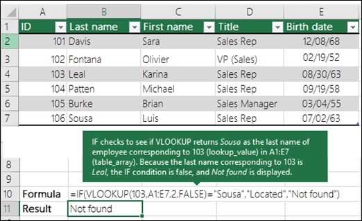
Alt text: Excel formula example using VLOOKUP within an IF statement, demonstrating conditional logic based on VLOOKUP result.

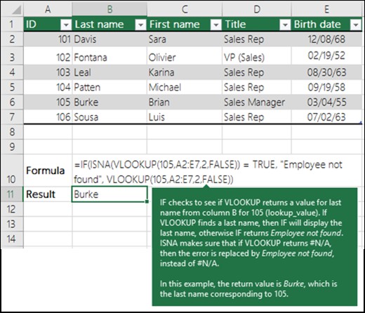
Alt text: Excel formula example using VLOOKUP with ISNA function to handle #N/A errors and return a custom value if lookup fails.

Problem	What went wrong
Wrong value returned	If `range_lookup` is `TRUE` or left out, the first column needs to be sorted alphabetically or numerically. If the first column isn’t sorted, the return value might be unexpected. Either sort the first column, or use `FALSE` for an exact match.
`#N/A` in cell	– If `range_lookup` is `TRUE`, and the `lookup_value` is smaller than the smallest value in the first column of the `table_array`, you’ll get the `#N/A` error. – If `range_lookup` is `FALSE`, the `#N/A` error indicates that the exact number isn’t found. For more information on resolving `#N/A` errors in VLOOKUP, see How to correct a #N/A error in the VLOOKUP function.
`#REF!` in cell	If `col_index_num` is greater than the number of columns in `table-array`, you’ll get the `#REF!` error. For more information on resolving `#REF!` errors in VLOOKUP, see How to correct a #REF! error.
`#VALUE!` in cell	If the `table_array` is less than 1, you’ll get the `#VALUE!` error. For more information on resolving `#VALUE!` errors in VLOOKUP, see How to correct a #VALUE! error in the VLOOKUP function.
`#NAME?` in cell	The `#NAME?` error usually means that the formula is missing quotes. To look up a person’s name, make sure you use quotes around the name in the formula. For example, enter the name as “Fontana” in `=VLOOKUP("Fontana",B2:E7,2,FALSE)`. For more information, see How to correct a #NAME! error.
`#SPILL!` in cell	This particular #SPILL! error usually means that your formula is relying on implicit intersection for the lookup value, and using an entire column as a reference. For example, `=VLOOKUP(A:A,A:C,2,FALSE)`. You can resolve the issue by anchoring the lookup reference with the `@` operator like this: `=VLOOKUP(@A:A,A:C,2,FALSE)`. Alternatively, you can use the traditional VLOOKUP method and refer to a single cell instead of an entire column: `=VLOOKUP(A2,A:C,2,FALSE)`.

Best Practices and Tips for Using VLOOKUP

To maximize the effectiveness and accuracy of your VLOOKUP formulas, consider these best practices:

Do this	Why
Use absolute references (`$`) for `table_array`	Using absolute references (e.g., `$A$2:$D$10`) when defining your `table_array` is crucial if you plan to copy or fill down your VLOOKUP formula to other cells. It ensures that the `table_array` range remains fixed, and doesn’t shift relative to the formula’s new position. Learn how to use absolute cell references.
Ensure data types are consistent	When searching for number or date values, verify that the data in the first column of your `table_array` is stored as numbers or dates, and not as text. Inconsistent data types can lead to VLOOKUP returning incorrect or unexpected results. You can use formatting tools in Excel to ensure consistent data types.
Sort the first column for approximate match	If you are using `TRUE` (Approximate Match) for `range_lookup`, always sort the first column of your `table_array` in ascending order. This is a strict requirement for approximate match to work correctly.
Utilize wildcard characters for partial text matches	If `range_lookup` is `FALSE` (Exact Match) and you’re working with text, you can use wildcard characters in your `lookup_value` for more flexible searching. The question mark `?` matches any single character, and the asterisk `` matches any sequence of characters. For example, `=VLOOKUP("Fontan?",B2:E7,2,FALSE)` will find “Fontana”, “Fontane”, “Fontani”, etc. To search for an actual question mark or asterisk, precede it with a tilde `~` (e.g., `~?` or `~`).
Clean your data	When working with text values, ensure the first column of your `table_array` is clean and consistent. Remove leading or trailing spaces, inconsistent use of straight (`'` or `"`) and curly (`‘` or `”`) quotation marks, and nonprinting characters. These inconsistencies can prevent VLOOKUP from finding exact matches. Use Excel’s `CLEAN` function or `TRIM` function to remove unwanted characters and spaces.

Beyond VLOOKUP: Consider XLOOKUP

While VLOOKUP is a fundamental and widely used function, Excel has introduced a more modern and versatile lookup function called XLOOKUP. XLOOKUP overcomes some limitations of VLOOKUP, offering improved flexibility and ease of use.

Advantages of XLOOKUP over VLOOKUP:

Searches in any direction: XLOOKUP can search to the left or right, unlike VLOOKUP which is limited to searching in the first column and returning values from columns to the right.
Defaults to exact match: XLOOKUP’s default match type is exact, making it safer and more intuitive.
More flexible syntax: XLOOKUP’s syntax is generally considered more straightforward and less prone to errors.
Handles missing values gracefully: XLOOKUP has an optional argument to specify a value to return if no match is found, eliminating the #N/A error in many cases.

If you are starting new projects or looking to upgrade your Excel skills, exploring XLOOKUP is highly recommended. However, understanding VLOOKUP remains valuable as it is still widely used and forms the basis for many lookup concepts in Excel.

Need More Help?

For further assistance and deeper exploration of Excel functions, you can always consult the extensive resources available:

Microsoft Excel Help: Use Excel’s built-in help feature by pressing F1 or searching in the help menu.
Excel Tech Community: Engage with experts and fellow Excel users in the Excel Tech Community.
Microsoft Support Communities: Get support and find answers in Microsoft Communities.
Online Tutorials and Courses: Numerous websites and platforms offer Excel tutorials and courses, including video demonstrations of VLOOKUP and other functions.

By mastering VLOOKUP, you’ll significantly enhance your data manipulation skills in Excel, enabling you to work more efficiently and extract valuable insights from your data.